Modifying Query in Powerpivot Report in Excel

Modifying Query in Powerpivot Report in Excel

In order to modify existing query in power pivot report in Excel 2010 and Excel 2013.

You have to follow below Steps

Excel Menu Bar

Go to Powerpivot tab

PowerPivot window

--This will open your existing query table

--Select the table in powerpivot window

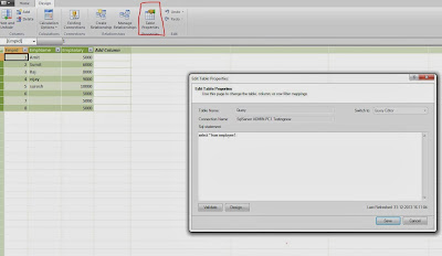
Go to Design Tab

click table Properties

Edit your query ( modify the query)

click save.

Screenshot 

Now go to Powerpivot excel Report.

Data

Refresh all 

It will Refresh the report with new Fields or Data.

Conditional Formating in Pivot Table Report in Excel 2010

Conditional Formating in Pivot Table Report in Excel 2010

While working with pivot table Report many times you have to apply conditional formatting to table,column or cell

for eg like if table or column has negative value make that color backround red.
if greater than 1000 then black
if equal to 500 then red and so on...

So in this post i will show how to apply conditional formatting in pivot table report in excel 2010.

Note: we will use the same pivot table which we have created in previous post

Creating Excel Pivot Table using SQL Database

http://sqlandssrssolutions.blogspot.in/2013/12/creating-excel-pivot-table-using-sql.html

so we will apply conditional formating in Salary Column like

if salary is equal to 10,000 then Darkyellow color text with light yellow background
if salary 9000 then redcolor text with light red background
if salary less then 9000 then greenbackground with bold text

For this select empsalary column

Go to home tab

conditional formatting

Higlight cells Rules

-Here you will find lots of options

-Greater then
--less then
--between
select the condition Equal to 
write  10,000 in first cell and in second cell some default custom is there apply 
Light red fill with Dark red background

 then apply other conditions.

Screenshot after applying condition format and options of condition format.

apply condition as mentioned above....

In condition format you can apply other conditions option like 

 Top Bottom Rules--for applying condition in top 10 or bottom 20 like this.
 Data bars- To convert your column to Bars.
 color scales - To apply coloring in cell and columns.
Icon set- In order to use indicators.

PowerPivot in Excel 2010

PowerPivot in Excel 2010

Below i will show to create a Pivot Table Report Using PowerPivot in excel.This is just a simple Report.

The Reason of using Power Pivot is it extends the capabilities of the PivotTable data summarisation and cross-tabulation feature with new features such as
expanded data capacity, advanced calculations, ability to import data from multiple sources, and the ability to publish the workbooks as interactive web applications.

Below are the steps of creating Power pivot Report in Excel

Open excel 
PowerPivot Tab
PowerPivot Window
--This will open a new window
Here we will create a report using SQL Database

-Select from Database
-ServerName
DatabaseName
-Next(screenshot)

-Here you wll get two options

-Select a list of Tables
-Write Query that will specify data to import

-So i will select from table
-next
-select table --you can select multiple table and can link them
--IT will create a Report for you with selected Table
Now click on pivot table
and insert a pivot table
In the Right hand side you will see pivot table fields

--YOu can add the column which you want to display in Report also you can add Slicer Directly like in the screenshot.

This is just a sample report so that anyone can get started with Powerpivot you can create Dashobards and many Complex reports using PowerPivot.

Displaying Pivot Table Column outside Pivot Table

Displaying Pivot Table field outside Pivot Table

In my Yesterday post i showed  how to display sum of Pivot Table column oustide Pivot table

In this Post i will show you  how to display pivot table field (Not Sum) outside Pivot table.

For This we have an excel formula GetPivotData.

We will use the Previous blog to create pivot table

Creating Excel Pivot Table using SQL Database

http://sqlandssrssolutions.blogspot.in/2013/12/creating-excel-pivot-table-using-sql.html

Slicers to Filter data of Pivot Table in Excel

http://sqlandssrssolutions.blogspot.in/2013/12/slicers-to-filter-data-of-pivot-table.html

Using the same above Pivot table and slicers to demonstrate the Solution to Display Pivot Table field outside Pivot Table.

Now suppose we want to display Raj salary  based on EmpName Raj salary (8000)

in Top row third fifth column i have to display Raj Salary so here is the formula 

=GETPIVOTDATA("Sum of EmpSalary",$A$2,"EmpName",A4)

Sum of Salary- Is the the pivot table column whose value to be displayed

$A$2-Cell of Pivot Table

EmpName-Is the column based on value to be displayed

A4-Is the Cell whose value to be displayed(Raj).

You can add Multiple fields data in GetPivottable by adding fields and item Name,

In order to display Grand Total outside Pivot Table Read my Previous blog.

Displaying Pivot Table Column Sum outside Pivot Table 

http://sqlandssrssolutions.blogspot.in/2013/12/displaying-pivot-data-sum-outside-pivot.html

Displaying Pivot Table Column Sum outside Pivot Table

Displaying Pivot Table Column Sum outside Pivot Table 

I was working on a Excel Report where i have to display the Grand Total of pivot table field in the Header of Report also  i was having slicer (Report filter ) in the Report.
Testing  Pivot Table and Slicers examples are in my Previous post.

Creating Excel Pivot Table using SQL Database

http://sqlandssrssolutions.blogspot.in/2013/12/creating-excel-pivot-table-using-sql.html

Slicers to Filter data of Pivot Table in Excel

http://sqlandssrssolutions.blogspot.in/2013/12/slicers-to-filter-data-of-pivot-table.html

Using the same above Pivot table and slicers to demonstrate the Solution to Display Pivot Table Sum outside Pivot Table.

Mistake What i did earlier in the Header cell i called the GrandTotal cell thinking that it was simple just to display the total.

like in below Report  c11  is the cell where i was having GrandTotal 53000 and i have to display the total
Salary in the first riw i.e Header.(c1)

so what i did in formula bar of C1 i directly wrote =C11(c11 is the cell displaying Grand Total)

It was displaying total correct until i didn't applied  filtered to the Report when i filtered the Report using Slicer it was showing Zero as Total Salary,which was 13,000.below screenshot.

Then i used GetPivotData function to display pivot table field but it didn't worked with GrandTotal for me.

So Here is the trick which i did for Solution .

write the formula =Sum(c3:c11)/2

--c2 is the first cell of the column from where to start summing 
--c10 is the last cell which has GrandTotal of all Salary.

Now add any filter to the Report it will show the Exact sum.

Note:Must  Include Grand Total cell in the Sum formula as final Range.

Slicers to Filter data of Pivot Table in Excel

Slicers to Filter data of Pivot Table in Excel

Slicer are used to filter the Pivot table in Excel slicers are the filtering component that contain a set of buttons
that enable you to quickly filter the data in a PivotTable report, without the need to open drop-down lists to find the items that you want to filter.
You can also add Slicers with  Olap cubes functions.(SSAS)

Slicers are same as Report Parameter in SSRS .

Below is the example how to add a slicer in the pivot table to filter the data.

if you want to know how to create a pivot table in excel then read my previous blog on
Creating Excel Pivot table

http://sqlandssrssolutions.blogspot.in/2013/12/creating-excel-pivot-table-using-sql.html 

we will add slicers to same pivot table which we created on our previous blogs.
.

we have 3 columns in our pivot table we will add slicers (empname and empid ) to filter the pivot table based on empname and empid

so below are step

First create a pivot table using the above link
click anywhere in your pivot table
Insert tab
click on Slicer
It will display all the column of your pivot table with checkboxes.
Select the checkbox for which you have to  add slicer in our case we are adding Empname and Empid

It will add two slicer in your Sheet.

Adjust the Position of Slicers.

click on any values of slicer to filter the report the Report will be filtered based on your values selection in slicer.

press Ctrl key with mouse click to add multiple values in slicer..

In order to clear all the filter from slicer click cross sign highlited in red in below screenshot.

Excel Report Hyperlink to Url

Excel Report Hyperlink to Url 

In order to add a hyperlink in a excel column create a excel sheet first like below sample data.with first two columns only.

Now in third column we will add hyperlink to site URL>

first column have site Name Second Column has Site URL now on Third Column we want the Name of Site and clicking on any Name in third column will open the Site URL. 

This is simple by hyperlink formula in Excel

Select your third column 3 rd row which is empty first 

click on fx 

Write formula
=Hyperlink(B2,A2) 

B2 is the value field which is url and A2 is the Name which we want to display. Writing formula will Automatically generate the site name with hyperlink to site URL.

Just Drag the formula field to all 5 rows of 3 rd column by clicking on plus sign..

Some play around with Hyperlink function.

The second argument of hyperlink function is optional if you will not give any value to second argument
it will take the first argument name which is url name eg

=Hyperlink(B2) 

Then site URL =http://sqslandssrssolutions.blogspot.in

and you can specify any name in Second argument of Hyperlink function.
like in last row i have use the formula

=Hyperlink(B2,"G") 

That's why it is displaying G not the site Name in row 6 of 3 rd column.

Now click on any site name in 3rd column will navigate you to corresponding Address.

Creating Excel Pivot Table using SQL Database

Creating Excel Pivot Table using SQL Database-Table

A pivot table is a data summarization tool found in data visualization programs such as spreadsheets or business intelligence software. Among other functions, a pivot-table can automatically sort, count, total or give the average of the data stored in one table or spreadsheet. It displays the results in a second table (called a "pivot table") showing the summarized data. Pivot tables are also useful for quickly creating unweighted cross tabulations.

Now in order to Create Pivot Table in Excel using SQL Database in SQL 

First create a table in SQL with Below Script

CREATE TABLE [dbo].[Employee1](
[Empid] [int] IDENTITY(1,1) NOT NULL,
[EmpName] [nvarchar](50) NULL,
[EmpSalary] [float] NULL
) ON [PRIMARY]
GO
SET IDENTITY_INSERT [dbo].[Employee1] ON
INSERT [dbo].[Employee1] ([Empid], [EmpName], [EmpSalary]) VALUES (1, N'Amit', 5000)
INSERT [dbo].[Employee1] ([Empid], [EmpName], [EmpSalary]) VALUES (2, N'Sumit', 6000)
INSERT [dbo].[Employee1] ([Empid], [EmpName], [EmpSalary]) VALUES (3, N'Raj', 8000)
INSERT [dbo].[Employee1] ([Empid], [EmpName], [EmpSalary]) VALUES (4, N'vijay', 9000)
INSERT [dbo].[Employee1] ([Empid], [EmpName], [EmpSalary]) VALUES (5, N'suresh', 10000)
INSERT [dbo].[Employee1] ([Empid], [EmpName], [EmpSalary]) VALUES (6, NULL, 5000)
INSERT [dbo].[Employee1] ([Empid], [EmpName], [EmpSalary]) VALUES (7, NULL, 5000)
INSERT [dbo].[Employee1] ([Empid], [EmpName], [EmpSalary]) VALUES (8, NULL, 5000)
SET IDENTITY_INSERT [dbo].[Employee1] OFF

Now open Excel 

---First we will create a Dataconnection to SQL Table for this below are the steps

Go to Data Tab 
Connection
ADD
Browse for More
New Source
SQL Server
-Connection Name
-Select your Database Name
-Select Table Name-Employee 1--above table which we have created
-click ok

Now in Order to create Pivot table

Go to Insert Tab
-Pivot Table
-It will ask for connection file
select the Name of connection file which we created above
click ok 

In excel you will see the the column Name in Right hand Side.

Drop EmpName and EmpID to Row Labels and Salary field to Values. It will Display Total Salary Based on  EmpID and EmpName.Its same as Group by in SQL displaying Sub total also.

IF you don't want subtotal of each EmployeeName Select your Pivot Table

 Go to Pivot Table tools-Design

-SubTotals

-Do Not show Sub Totals

You will have your Pivot table displaying Employee Name ,ID and Sum of Salary.

Searched Case Expression in SQL

Searched Case Expression in SQL

The CASE expression has two formats:

The simple CASE expression compares an expression to a set of simple expressions to determine the result.

The searched CASE expression evaluates a set of Boolean expressions to determine the result.Like it Searches for condition and based on that it display Data

Example explaining Searched case expression

 In below Table we have Empsalary field it will check for Salary if Salary is 5000or 60000 it will double the salary in the output and if empname is null then it is returning salary as zero

--Table with employee Detail and Salary

CREATE TABLE [dbo].[Employee1](
[Empid] [int] IDENTITY(1,1) NOT NULL,
[EmpName] [nvarchar](50) NULL,
[EmpSalary] [float] NULL
) ON [PRIMARY]
GO
SET IDENTITY_INSERT [dbo].[Employee1] ON
INSERT [dbo].[Employee1] ([Empid], [EmpName], [EmpSalary]) VALUES (1, N'Amit', 5000)
INSERT [dbo].[Employee1] ([Empid], [EmpName], [EmpSalary]) VALUES (2, N'Sumit', 6000)
INSERT [dbo].[Employee1] ([Empid], [EmpName], [EmpSalary]) VALUES (3, N'Raj', 8000)
INSERT [dbo].[Employee1] ([Empid], [EmpName], [EmpSalary]) VALUES (4, N'vijay', 9000)
INSERT [dbo].[Employee1] ([Empid], [EmpName], [EmpSalary]) VALUES (5, N'suresh', 10000)
INSERT [dbo].[Employee1] ([Empid], [EmpName], [EmpSalary]) VALUES (6, NULL, 5000)
INSERT [dbo].[Employee1] ([Empid], [EmpName], [EmpSalary]) VALUES (7, NULL, 5000)
INSERT [dbo].[Employee1] ([Empid], [EmpName], [EmpSalary]) VALUES (8, NULL, 5000)
SET IDENTITY_INSERT [dbo].[Employee1] OFF

select * from Employee1

--Query Displaying Empdetail with different conditions

select case when empsalary =5000 and EmpName IS not null then '10000'
when EmpSalary =6000 then '12000'
when empsalary=5000 and EmpName is null then '8000'
else empsalary end Salary
,EmpId,Empname from employee1

If you want to know about simple case expression with examples read my post:
http://sqlandssrssolutions.blogspot.in/2013/07/introduction-to-case-statement.html

Fetching Excel Sheet Data in SQL using SQL Query

Fetching Excel Sheet Data in SQL using SQL Query 

In order to Select, fetch or Read  the Excel Sheet Data using SQL Query or Creating Table in SQL  using Excel query first configure the advanced option through below scripts

step 1
sp_configure 'show advanced options', 1;
RECONFIGURE;

step 2
sp_configure 'Ad Hoc Distributed Queries', 1;
RECONFIGURE;
GO

Step 3


for MSExcel 2007 and 2010 --Database is the path of your excel sheet ,sheet1 is the name of sheet1

SELECT * FROM OPENROWSET('Microsoft.ACE.OLEDB.12.0', 'Excel 8.0; Database=E:\book2.xlsx', 'SELECT * FROM [Sheet1$]');


Step 4 if you want to create a new table in sql based on excel data
for MSExcel 2007 and 2010 --Database is the path of your excel sheet ,sheet1 is the name of sheet1

SELECT * into test FROM OPENROWSET('Microsoft.ACE.OLEDB.12.0', 'Excel 8.0; Database=E:\book2.xlsx', 'SELECT * FROM [Sheet1$]');


Case if you are using Excel 2003

SELECT * FROM 
OPENROWSET('Microsoft.ACE.OLEDB.4.0', 'Excel 4.0;Database=E:\book2.xls;HDR=YES', 'SELECT * FROM [Sheet1$]');


 In case if you will get error like 

Msg 7308, Level 16, State 1, Line 1
OLE DB provider 'Microsoft.ACE.OLEDB.12.0' cannot be used for distributed queries because the provider is configured to run in single-threaded apartment mode.

Run the below script to fix the Error

EXEC master . dbo. sp_MSset_oledb_prop N'Microsoft.ACE.OLEDB.12.0' , N'AllowInProcess' , 1
GO

EXEC master . dbo. sp_MSset_oledb_prop N'Microsoft.ACE.OLEDB.12.0' , N'DynamicParameters' , 1
GO

Note: You can use import export wizard ,SSIS also to import Data from excel sheet to sql

Incorrect Paging in SSRS Report

Incorrect Paging in SSRS Report

While Creating a SSRS Report one of my friend Faced problem like he has some records in his report which were coming in two pages of SSRS Report.

But the Total no. of pages in the report was showing 3 and opening 3rd page was completely blank with no records which was of no use so he don't want to have 3 rd page in Report.

Below screenshot with Empty Records last page.

Solution

I checked the Report the Reason was like the size of Report body was greater then Report size so i changed the Report body to 2 inches

and Report size  to 10 inches 

Preview the report 

Now Report was showing only 2 pages which was Required.

now there was no extra page issue in the Report.

Note:Always keep the Size of Report body less then Report to avoid these types of issue.In order to know how to fix Report body and report size read my post on Report size.

http://sqlandssrssolutions.blogspot.in/2013/12/how-to-fixheight-and-width-of-ssrs.html 

SQL Facts and History

SQL Facts and History

As this is my 100 post on my blog so i thought to write some  interesting Points about SQL.

1-SQL stands for Structured Query Language. SQL is a standard language that was designed to query and manage data in relational database managementsystems (RDBMS).

2-It is a database programming language(TSQL) that acts as a means of communication between two other programs such as a Webapplication and a database.

3-The relational model is language-independent. That is, you can implement the relational model with languages other than SQL.

4-SQL was initially developed at IBM by Donald D. Chamberlin, Donald C. Messerly, and Raymond F. Boyce in the early 1970s called SEQUEL (short for Structured English QUEry Language) for their RDBMS product called System R. 

5-The name of the language was later changed from SEQUEL to SQL because of a trademark dispute.

6-Major component of SQL DDL,DML and DCL.

7-Examples of some  websites that use SQL in some capacity are Ebay, Microsoft and Amazon.

8-SQL is not a case sensitive language.

9-SQL is a Product of Microsoft.

10- Microsoft SQL Server, has several add-on services that manage different aspects of enterprise business intelligence and information processing such as data integration, reporting and analysis(SSRS SQL Server Reporting Service ,SSAS SQL Server Analysis Service,SSIS SQL Server Integration Service).

IF Else Condition in SQL

IF Else Condition in SQL 

The IF Else condition in sql allows us to control the flow of our sql code or query.
For example the below if else condition shows that if current date is greater then 15 of the month then it will show
Fee pending please pay the fees
else It will show 'you have paid your fees'


if day(getdate())>15
print 'Your fees date is over please pay the Pending fees'
else
print 'you have paid your fees'

Output--as today date is 16 december greater then 15
Your fees date is over please pay the Pending fees

IF you want more condition to be added you can you else if statetement or case statement.

Syntax else if

IF condition1..
result1
else if  condition2...
result2
else condition2...
result

Syntax case 
Case when condition1 then result1
Case when condition2 then result 2
else result3 end

How to Fix Height and width of SSRS Report

How to Fix Height and width of SSRS Report

A conman mistake is like in order to fix height and width of report some users use to change height and width of body of Report and faces the problem that while preview the report the report height and width is not getting fixed. 

So,In order to fix or set SSRS Report Height and width 

Right click outside the report.

select Report properties.

set Height and width of Report.

Click ok. 

Preview the Report the Report size will be fixed.

Note: In case where your table size is more then Report size then first you have to fix the Table height and width and then Report Size.